
Key Points
- A clear understanding and estimation of an asset’s remaining useful life is challenging but extremely advantageous to industrial operators
- RUL enables operators to optimise maintenance, de-risk operations, manage spare parts and generally improve awareness of system health
- Machine learning models can associate the degradation mechanisms of complex industrial systems to an estimate of RUL in cycles or uptime
The Benefits of Understanding RUL
RUL or remaining useful life is an estimation of the leftover time or cycles that an industrial asset or system can operate successfully. A function of system age, machine health and scheduled future use, RUL can be considered the time until critical failure or a level of degradation is reached, severe enough that the system can no longer function up to an acceptable quality or capacity.
OEM’s often guarantee healthy operation up to a certain value but offer no operational advice beyond this threshold, leading to variation in observed asset life span. When there is high uncertainty in the expected lifespan of a critical system or asset, developing an understanding into the remaining useful life of the system is critical for O & M practices, preparation, and risk optimisation.
RUL prediction can provide insights and benefits such as:
- Provision of advanced condition monitoring, enabling informed system inspection and prognostic insights
- Support of warranty claims for critical and expensive system assets against OEM providers
- Enable optimised supply and demand management of spare parts through the insight gained into the RUL of a dependent system
- Sizeable maintenance optimisation possibilities through prevention or prioritisation across a fleet of repeated assets such as a wind or solar farm
RUL is most beneficial when applied to equipment with a gradual degradation process such as rotating plant and with high variability in its life expectancy.
The Data Driven Approach
There are many approaches to deriving an estimate of system RUL. Methods from the physical science domain, statistical methods such as survival analysis, and data driven regression-based techniques implementing machine learning.
The data driven approach is by far the most flexible as it is capable of incorporating contextual and instrumentation data as well as embedding information obtained from the system’s life span. There is no requirement to have an accurately defined dynamic model of the system and its degradation process, instead these underlying behaviours are learned from historic data using advanced AI.
Example: RUL of a Turbine Engine
This open-source data set is commonly used for the development and testing of RUL methodologies. https://data.nasa.gov/dataset/C-MAPSS-Aircraft-Engine-Simulator-Data/xaut-bemq
The training data consists of complete operational histories for a number of turbines, each made up of individual runtime cycles. Sensor data is recorded within each cycle of the turbine lifespan from a series of 24 unique sensors. The modelling goal is to relate the historic sensor data to the RUL of the turbine, cycle by cycle.
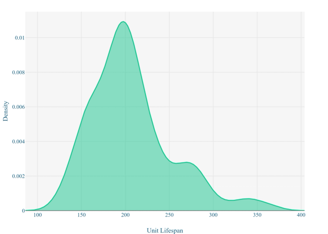
Figure 1 shows the distribution of lifespans for the complete set of turbine, there is high variance in the magnitude of these life spans and covering a significant range. This observation suggests there is substantial value in developing an RUL predictive model for this use case. Using the observed lifespans alone may lead to the development of a conservative O&M strategy suggesting an early turbine replacement (e.g., at 100 cycles), which in many cases would be wasteful.
To predict RUL, we assume that the sensor data contains some concealed information or pattern which relates to turbine health or a level of degradation and can be extracted to serve as a system health indicator. Which, in turn, can be associated to the RUL.
Using deep learning methods, we can combine these two distinct stages in the modelling process. Neural networks such as 1d-CNN’s or LSTM’s will learn within the training process to detect features that express degradation behaviour and relate this to the underlying RUL of the system.
Instead of trying to predict the linear RUL as a number of remaining cycles, it may be more sensible to mutate it to better reflect the expected degradation process of the system. By predicting the raw observed RUL directly, we make the assumption that the equipment decays linearly throughout its lifespan. However, this degradation model is uncommon, in the case of the turbine it is suggested that the equipment decays in a piecewise linear form. Implying that the system undergoes little to no degradation in its early life before an event occurs which triggers a linear degradation process from then onwards. To incorporate this domain knowledge within the modelling process, the linear saw-tooth RUL variable is transformed to reflect the piecewise degradation process. This is achieved by capping the RUL observations to a maximum number of cycles, creating a blunt saw tooth shape, Figure 2.
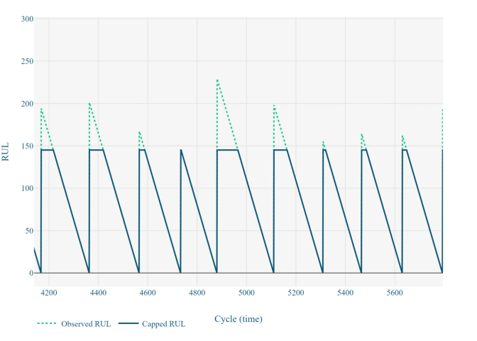
This transformation should enable the neural network architecture to better relate the sensor data to the degradation process and improve the prediction accuracy. It is important that this transformation is communicated to the end user, as it may be confusing to install a new turbine and have the predicted RUL seem lower than the average equipment life expectancy.
The Modelling Process
Using a 1d-CNN it is possible to pass a sequence of time series data as a predictor, this is combined with the age of a target turbine as the features used to predict the RUL.
The model is trained over 100 turbine life spans leading to a total of >17,000 RUL observations. The best model was selected by MAE over an out-of-sample data set. It may be more suitable to select a performance metric which penalises late predictions more heavily than early ones.
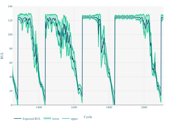
The model achieves an average percentage error of ~10%. From Figure 3 we can see that the model often predicts with low uncertainty around the turbine’s initial life span. This justifies the piecewise linear assumption. If this degradation model was not a good fit, we would expect to see high uncertainty around the early system life in particular, as well as an overall higher MAE. This would be due to the model being unable to relate a discovered degradation signal in the sensor data to an unchanging RUL label.
Conclusion
The development of digital twin technology that can accurately assess recent system operation and estimate RUL can enable significant industrial improvement. In the case of the turbine an accurate predictive model can be developed, allowing for the development of dynamic and optimised maintenance strategies. Spare or replacement turbine engines can be commissioned in time, maintenance teams can be arranged, and their activity can be optimised. Intervention can be carried out to prevent system failures which will improve uptime, prevent damage to neighbouring systems and increase safety.
The requirement for complete system life span data appears to be a hard barrier at first glance. O&M strategies rarely allow critical systems to run to failure. This censors the complete system lifespan and hence prevents the collection of the RUL labels. However, there are ways around this problem. The definition of when a system is no longer usable can be adjusted to fit data requirements. For example, a system may be scheduled for replacement on the outcome of a maintenance inspection, at this point in time the system can be deemed as no longer useful, providing a label. Alternatively, it may be possible to define a threshold or alarm in breach of which the system is expected to no longer be of service, hence providing a label. Using these problem reframing techniques, the journey to complete RUL transparency can begin.